I’ve recently covered Oeksound Soothe, and now it’s time to check out their other product: Spiff.
Unlike Soothe, I’m less skeptical going into this one. I’m also intrigued by the concept of an transient controller. Let’s jump in now, once again with a minor aside…
Contents
Video
It’s a sad story, but one that must be told.
Precursor
FFT
Step one here is to head back over to the Soothe post and make sure you’re familiar with some basic concepts. To fully understand how Spiff works, you need to have a base idea of these concepts.
Transients
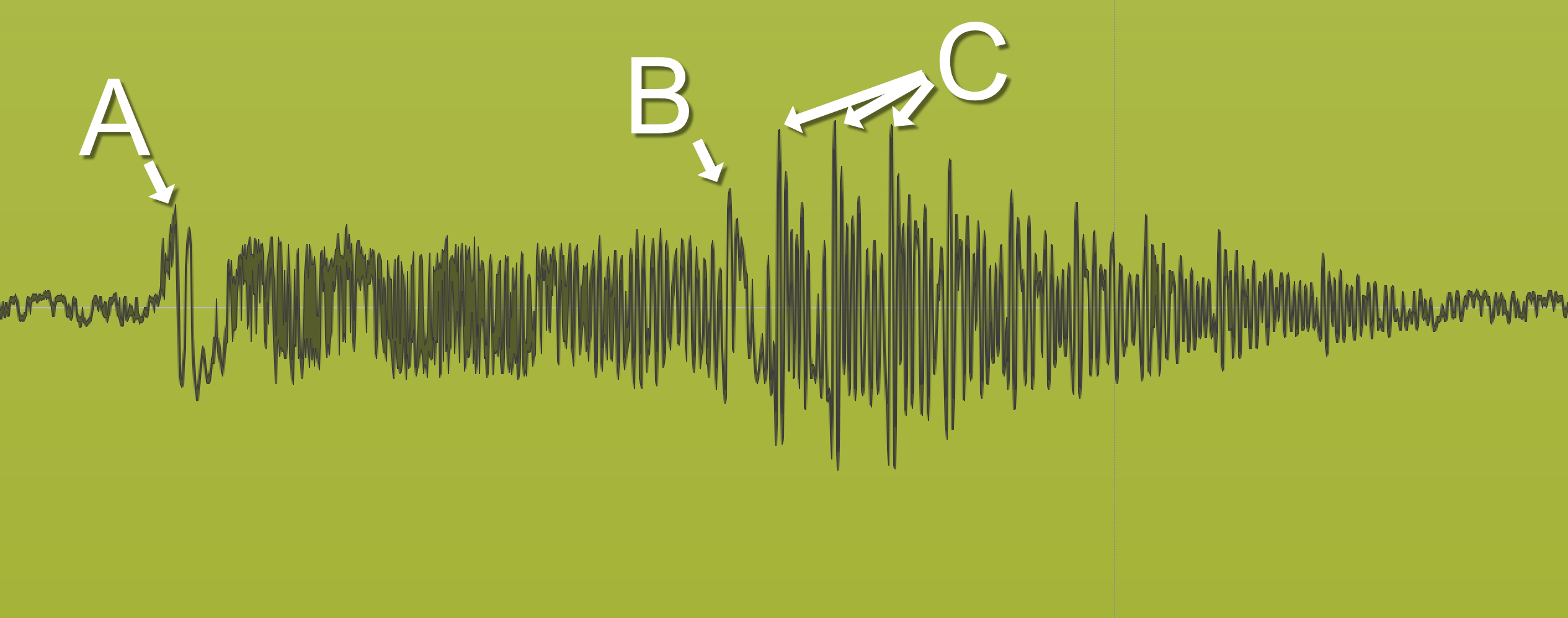
We need to take a moment to talk about what a transient is. So in the image above, which one is a transient? A? B? C?
- A - yep. Transient.
- B - affirmiative. Transient.
- C - 예. Transient… maybe.
I bet that a number of people reading just thought A was the transient, but no matter how we define transient we have to include both A and B. Sure we could create an algorithm that somehow detects only A, or A&B or only C or only A and C… but it wouldn’t be a useful transient detector.
Let’s go with this concept of a transient: A transient is a sudden change in energy.
SUDDEN. Think about that word. That means that it happens quickly. If we wish to speak in terms of “frequency”, we would say that it’s a high-frequency change.
That makes life a bit difficult as a DSP-dude. We roll along calculating the ‘current energy’ of a signal and label something a transient when there’s a fast jump. If we do this naïve method then we’ll only detect high-frequency transients. Using such an algorithm we’d catch A and B, and C depending on how sensitive the algorithm is. That usually works ok if you’re just trying to handle musical concepts.
But what about words? If you have a microphone, record yourself saying “Hi” in an abrupt fashion. You open your mouth and blast out a breath of air. It looks like this:
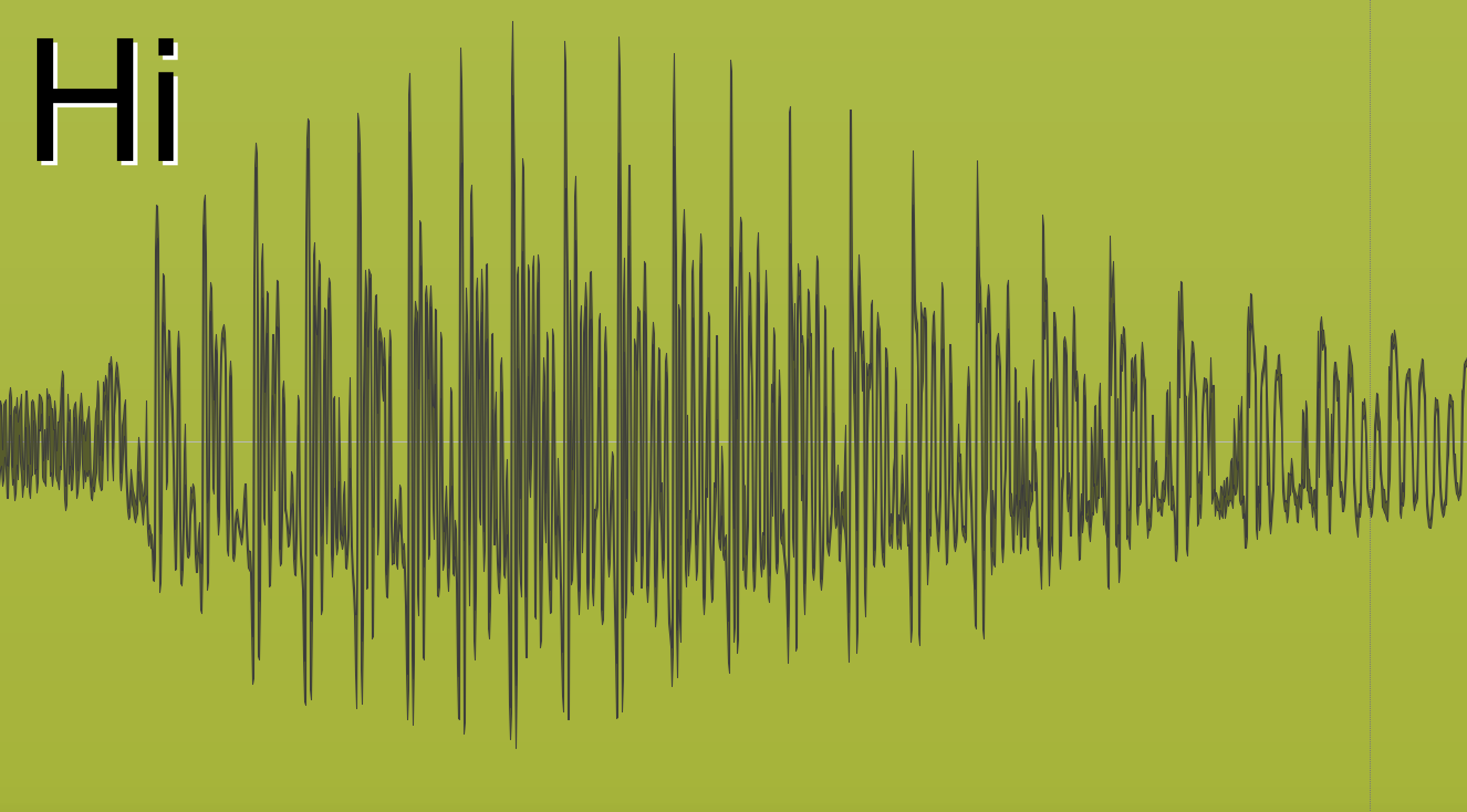
What do we see here? It is a mostly low-frequency, with a little bit of a high-frequency sound interwoven. The important thing that we need to recognize here is that there is no obvious “transient”.
What we have is a slow ramp-up until we hit the top of the “H” sound.
How do we determine where the transient is in the sound. If we use our concept of ahigh-frequency event then it won’t work, because we have a slow amplitude ramp and a mostly low-frequency sound.
That is where the FFT comes in. What if for each frequency bin in the FFT we adjust what we consider a “sudden” event. Something that is sudden in a low-frequency bin happens a bit slower than something that happens in a high frequency bin.
I’m going to leave you with that thought, since that’s how things like Spiff work.
FFT size
As was discussed before, the FFT is a transform that let’s us extract ‘frequency data’ from a bunch of samples. What we didn’t discuss is how the human ear hears things, and what this means about the FFT.
Musically, we tend to hear things in octaves with notes spaced between them. How those notes are spaced between octaves is an entirely different topic. So if you play the note C, then play a C that is just “one step” higher in pitch, then you’ve played an octave.
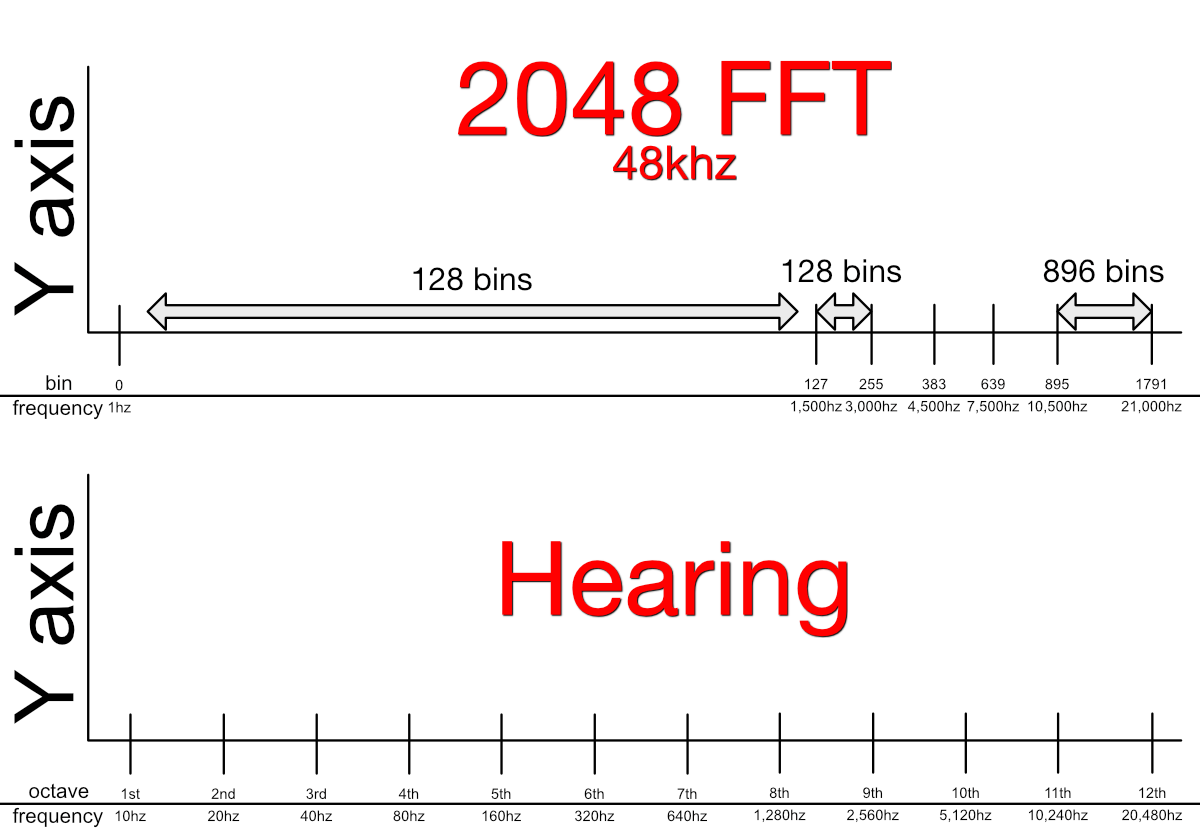
What is important to recognize here is that an octave is a doubling in frequency. Look at the bottom graph in the image above. We start with a note that is at 10hz. Each time we go up an octave, we double the frequency of our current note. So we go from 10->20, then we double 20 to get to 40. Now we double 40 to get to 80, etc…
Our response to frequency is logarithmic. (So is our response to amplitude… another post, again.) By time we get to the 11th octave we’ve long maxed out the average adult’s hearing range.
The FFT isn’t logarithmic. It splits the sound into bins, and these bins represent an even split of the available bandwidth. So if we’re at 48,000hz sample rate, we can represent a sine wave up to 24,000hz. With an FFT window size of 2048, that means each bin is separated by 24,000 / 2048 = 11.71875hz.
That’s a BIG ISSUE for us! Look at the top graph now.
Each 128 bins spreads about 1,500hz (24000 / 2048 * 128). It’s linear (evenly spread). Our “first bin” (0) is set at 1hz in this example. 128 bins to the right, we’re at 1,5000hz.
1/16th of our available FFT bandwidth is EIGHT OCTAVES. 1/16th of our FFT is 8/11ths of our audible hearing. That’s a terrible ratio.
To think of that another way, we have 128 bins to represent over 8 octaves. The remaining 1,920 bins represent the remaining 2.5 octaves. Ugh. Ouch. BlErGh.
Now the curious engineer already has experienced this. You look at your sound in an FFT-based analyzer and the low-end has terrible resolution, but the high end is more defined than the finest of ginsu knives (Yes I remember those commercials as a kid.)
The FFT algorithm that most audio products use depend on windows based on powers of 2 (Explaining this is another post… again). So if we want more resolution then we go from 2048 (2^12) to 4096 (2^13). Now we have 256 bins that spread our over 8 octaves. Much better! Still not great.
So you’d think, “Robert, this is a simple task. I’m just going to use an FFT window of 2^24 (16,777,216) and then I will be king of the frequency spectrum!
Not so.
FFT and Transients (Overlap again)
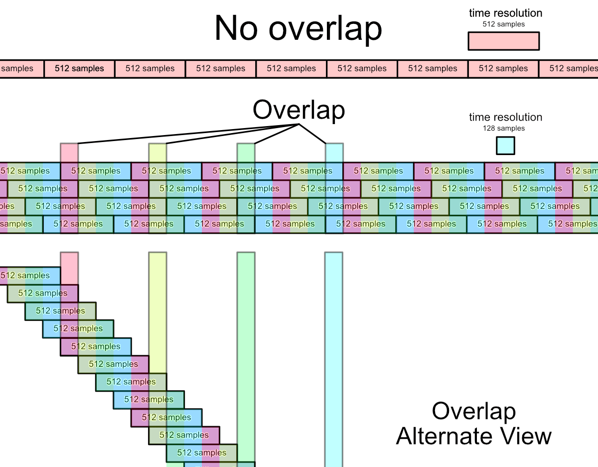
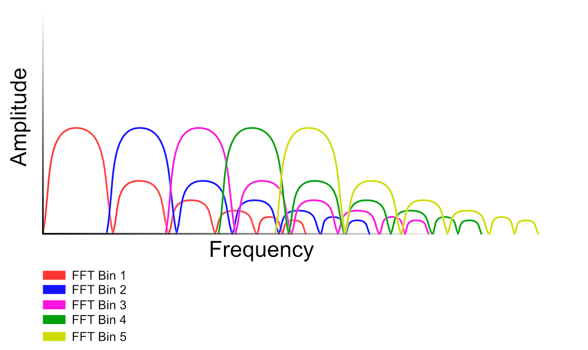
This should be a familiar graphic. What you should understand is that how fast we get data back from the FFT depends on the size of the FFT. Larger FFT’s mean we get data back much more slowly.
But we can cheat.
If we send out an fft more often than we get data back, we can get data back more often. Maybe that sounds weird, let me try again: if we have a 1024 sample FFT and we calculate an FFT every 256 samples, we can get data back 4x as fast.
We also use 4x the calculations, because every 1024 samples has 4 fft processes going.
Cheaters always lose in the end, I suppose.
Like everything in audio, there’s tradeoffs. If we want massive frequency resolution then we pay for it with time resolution. If we want to buy more time resolution then we pay for it with processing power (and some other factors).
Linear Phase Tradeoffs
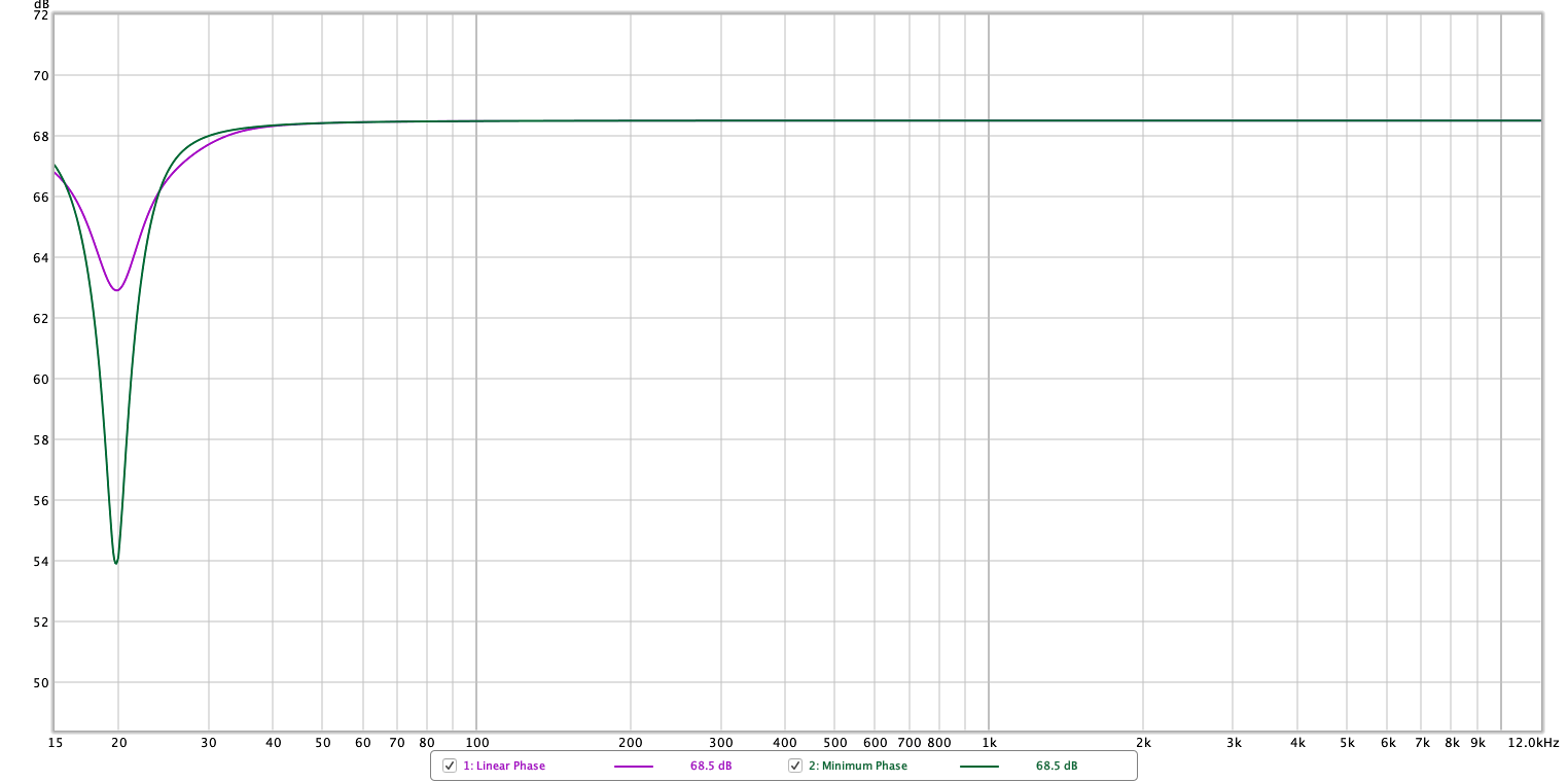
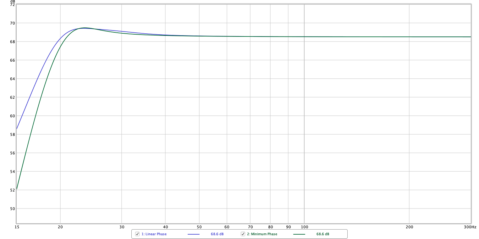
This is the same filter implemented in linear phase and minimum phase versions. (Note that the X axis is changed in the second graphic).
These graphs demonstrated the unfortunate fact that linear phase filters have some “difficulty” in reproducing similar accuracy with low frequencies. This is rather important!
Likewise, the concept of “pre-echo” is important to understand.
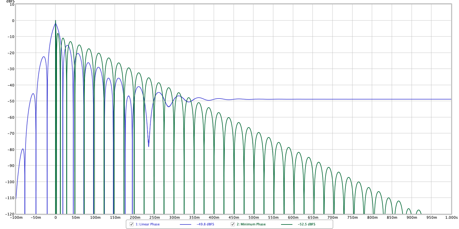
Above is a step response graph. It’s similar to impulse response, but cleaner to look at. Impulse Response is 0’s followed by a single sample of >0 value then 0’s again. Step response is 0’s followed by a sudden change to all 1’s.
The X-axis here is time. The green minimum phase filter starts ‘making noise’ at 0ms and then infinitely decays until it disappears into the precision threshold of our data type. (Until it’s below the noise threshold).
The blue linear phase starts before 0ms. That’s right! When using a linear phase filter, we will hear some sound before the sound happens. With this filter we will hear a fairly significant pre-echo -22dB below our signal at about -30ms. That’s a pretty big deal. It makes a kinda weird “Ba-dum” (flam) sound if you were to use this on a kick drum.
That’s not all bad though. The linear phase filter is linear phase. There is no phase rotation for reasonable uses, so it has a somewhat more pleasant sound with sudden and large changes. It also plays nicely with parallel processing (what happens if part of your signal is 180° rotated and mixed in? That doesn’t happen with linear phase).
Energy
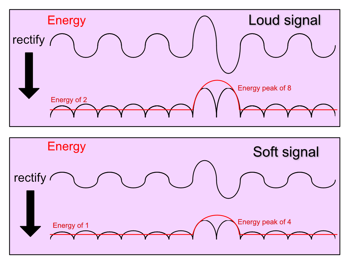
Transient processors tend to work on some concept of energy.
First you take your signal, which goes from -1 to 1, and take the absolute value of every sample. This is called rectification. Now you have a signal that you can sort of ‘see the envelope’.
Now you use some fancy algorithm to determine the amount of energy in the signal over time. Remember that sound is pressure, which translates nicely to the concept of energy. The representation of sound in your DAW can be turned into some representation of energy.
With a representation of the energy in the signal, you can now look at the relative changes over time. If there’s a big change then YAY!, it’s a transient.
The beauty of this is that you’re looking at relative changes. In our example above, even though our loud signal is twice as loud, the relative change in energy in that peak is 2:8, or 1:4.
With a signal that’s “half as loud”, our energy ratio becomes 1:4.
The peak has the same ratio of energy change. Our processor is level independent. Unlike a compressor, the level of the signal in our transient processor does not affect when the processor acts.
Now take this concept and apply it to FFT based analysis. Instead of looking at the changes in energy for the whole signal, you have 100s or 1,000s of bins that you can analyze their level.
Another neat thing about working with FFTs is that you can normalize them. Find the bin with the highest value, turn it up till it’s 0dbFS and then turn up all of the other bins by the same amount. No matter what the level is, your frequency analysis always has a peak at 0dbFS. This gives you another level of level independence.
IMPORTANT Does spiff work this way exactly? I’m not 100% sure. The core concept applies, but there’s a lot more to it as you’ll see.
There are other ways to detect transients, but the level independent processors (like Spiff) all work around this core concept. (Even if it’s more complex, the base idea remains)
I am explaining this so that you understand how it’s different from a threshold based processor such as a compressor or Soothe
Spiff Basics
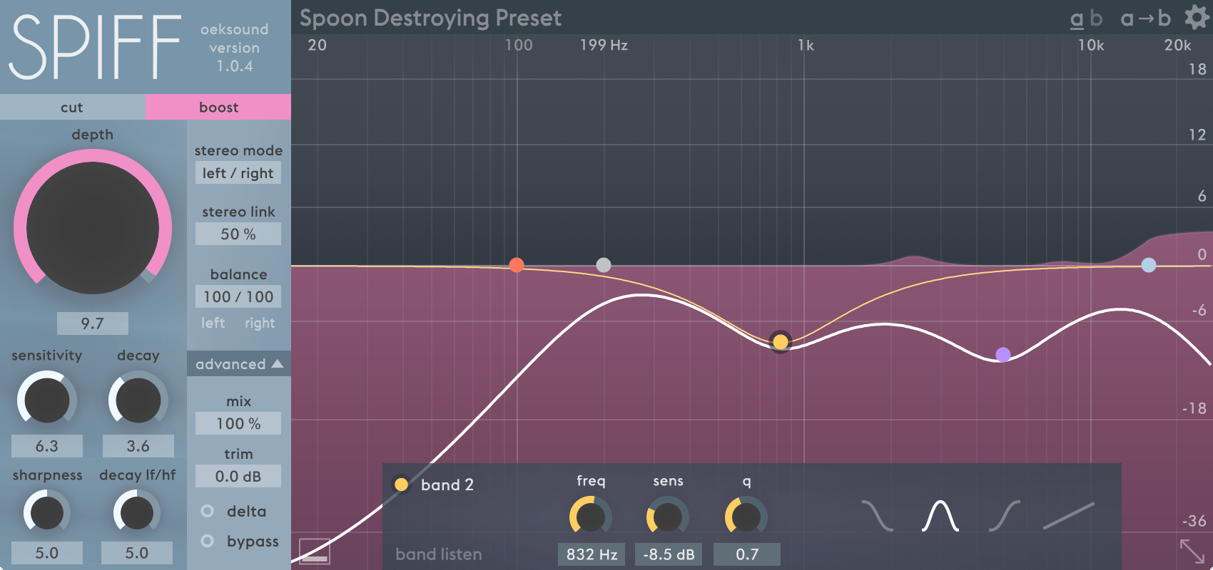
Left Panel
On the left panel you have some familiar controls if you’ve used or seen Soothe, but there’s some twists in this story:
- Boost/Cut - Spiff works in one of two modes, a boost or a cut mode. This is where you select which mode it is operating in. It does not operate in both modes simultaneously.
- Depth - Depth is a bit more complicated on Spiff compared to Soothe. As far as I can tell there isn’t a ‘threshold’-like behaviour in the direct sense, but instead a multiplier of how much processing should be applied.
- Sensitivity - The sensitivity knob changes how reactive Spiff is to energy changes.
- Sharpness - This is the width of the filters
- Decay - Spiff does not react to a well-defined threshold. There is no clear-cut concept of when an event has ended. So you can set how long the filters take to reset to zero after a transient event has happened.
- Decay lf/hf - Remember how we discussed the concept that high frequencies are more likely to be transient? Since Spiff attempts to detect transients in all frequency ranges, it is potentially necessary to relax the filters to zero at different rates. Moving the knob to the left makes low frequencies decay slower, and moving the knob to the right makes high frequencies decay slower.
Right Panel - Part 1
- Stereo Mode - The stereo mode allows you to switch between the normal left and right mode, and mid/side mode. Mid/side mode allows Spiff to process audio that is identical between the channels separately from audio that is different between the channels. What this is set to affects the stereo link and balance controls.
- Stereo Link - Stereo link at 0% allows Spiff to work on each signal independently. At 100% it applies the same processing to both signals. This is particularly interesting when using the mid/side mode. Spiff can apply processing to the mid-channel and side channel separately, which is extremely useful when working with things like stereo drums or other stereo musical sources.
- Balance - This is not just a left and right hand, but it also lets you change the proportions between the mid inside signals. If you wish to turn down your phantom center (the mid-channel) then you can adjust the balance as shown. When stereo mode is set to mid/side the balance control is value/value. A value of 100/0 processes only the mid-channel. A value of 0/100 processes only the side channel.
- Resolution - Resolution adjusts the amount of overlap. Normal = 4x (75%). High = 8x (87.5%). Ultra = 16x (93.75%).
- Oversample - Oversampling allows the filters to be more precise in both the time and frequency domains.
- Window - This changes the size of the FFT Window.
- Phase Mode - Linear and Minimum phase filter selection. Minimum phase is preferred for low-frequency work, and linear phase otherwise.
- Mix - This lets you blend the process signal with the original signal.
- Trim - Trim is the output volume control.
- Delta - Delta is a need control that allows you to listen to only what Spiff has done to the signal. Extremely useful for initial setup.
- Bypass - This is bypass. It turns off the processing.
Right Panel - Part 2
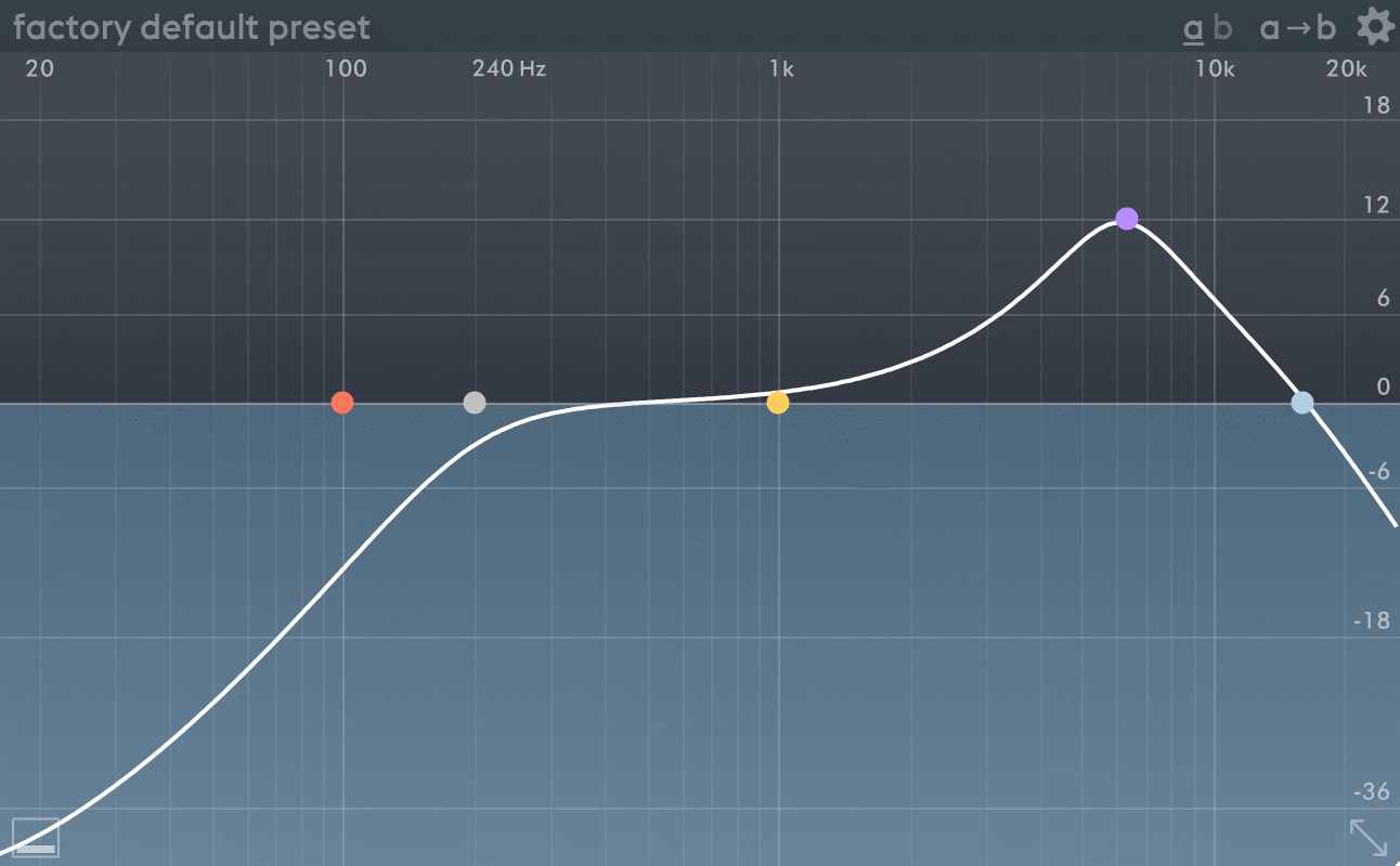
Just like Soothe, Spiff allows you to adjust the signal that is being used to make processing decisions without actually touching the signal that is being processed.
You can think of this as a sidechain equalizer.
Spiff has a much more feature full equalizer section compared to Soothe. You are not locked into a specific band type per node on the 3 middle bands. The low/high pass have 4 slope settings (I assume between 1-4 pole? (6-24dB/octave)). The other bands:
- Low/High Shelf - Shelving filters which reduce everything to the left (low) or right (high) equally after the transition.
- Bell - Your normal biquad bell.
- Tilt - This is a neato filter type. It’s simultaneously a low and high shelf. You can control both the bands to the left and to the right of the node and low/high shelving filters are inversely proportional to each other in amplitude. If you make it boost to the left of the node, it will cut to the right. If you cut to the left of the node, it will boost to the right.
Another extremely cool feature is “Band Listen”. You can solo only the frequency range of the width of the band that you are working with to make changes more effectively. The tilt filter band listen solos the transition between the low and high shelves.
Yet another feature that Spiff has over Soothe (as of this review) is an A/B system. You can store settings in the A slot, then store a another setting in the B slot and quickly move back and forth between them. There is also the “A->B” button that allows you to copy your settings from the A slot to the B slot.
Testing
Sine Sweeps
Nope. Not today. This is a transient processor. Even if you try to be clever by using single sine wave cycles, you won’t get good results.
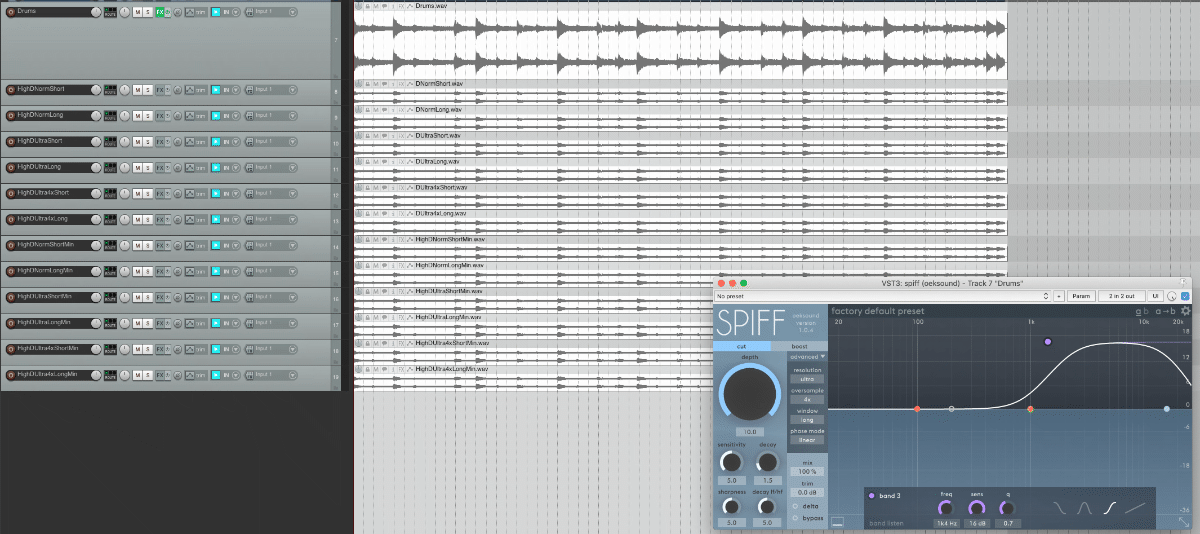
Resolution, Oversampling and Window
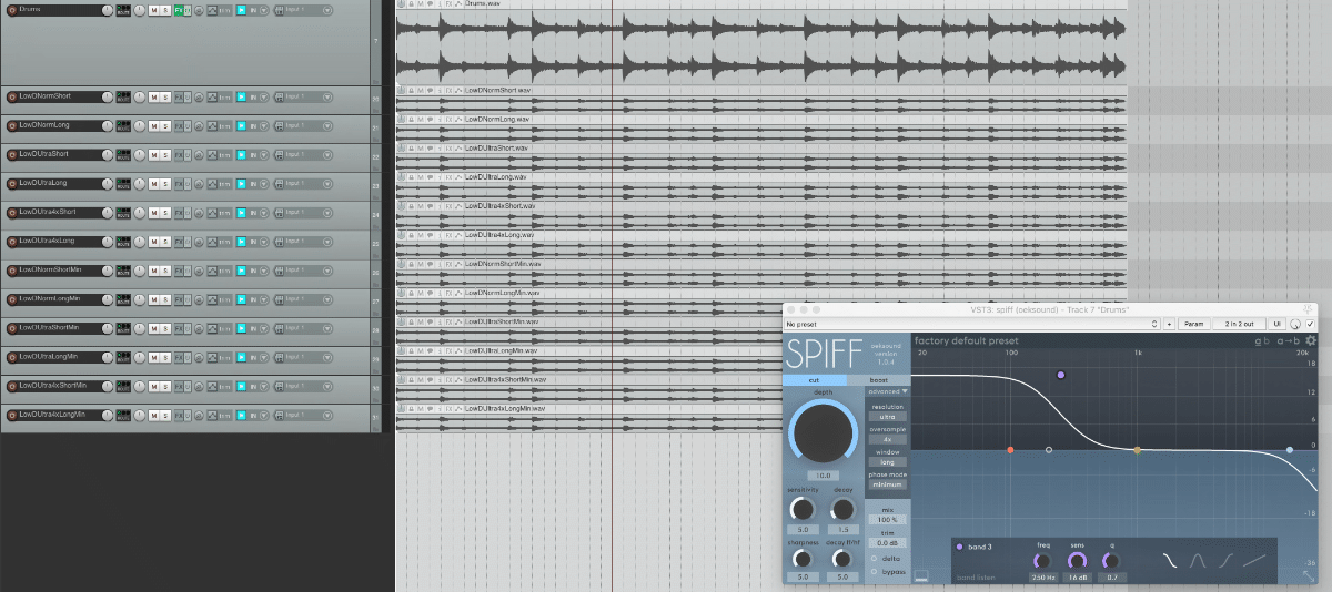
The question here is if it’s worth using the higher values of the Resolution, Oversampling and Window controls. For this test I’m using a drum loop.
I will render each combination of settings then attempt to sum those settings with the inverse of another set of settings. There will be two tests: low frequency and high frequency. I be using the cut mode.
I will only be using the extremes of the settings so I don’t end up with 50+ files to test.
Here is the file used for testing. I tried to make sure it was a somewhat complex recording with variance between low and high frequency parts.
IMPORTANT These tests don’t show what the audible difference is. You won’t learn what the sound difference is that you hear, only how much of a difference there is.
The files also were not normalized, so the absolute value does not matter. Only the relative difference matters.
High Frequency - Cut
This is a test with a focus on higher frequencies. This is not an exhaustive test by any means, and I know for a fact that I can create pathological examples to create larger differences. I decided to use a ‘real world’ test instead.
Higher numbers indicate a bigger difference between the two compared settings. Normal/Ultra is the resolution setting and Short/Long is the Window size.
| Normal Short | Normal Long | Ultra Short | Ultra Long | |
| Normal Short | X | -15.9 | -32.4 | -15.0 |
| Normal Long | -15.9 | X | -16.4 | -18.6 |
| Ultra Short | -32.4 | -16.4 | X | -15.0 |
From this test we can see that when using longer window sizes seems to make the biggest difference. Like Soothe, the resolution setting makes a relatively minor difference.
Oversampling is shown here using the ultra resolution with varying windows and oversampling:
| Ultra Short 4x | Ultra Long 4x | |
| Ultra Short | -32.3 | -14.2 |
| Ultra Long | -15.3 | -29.8 |
There’s not much of a difference in oversampling in this test. Changing the window size has a significantly larger difference.
| Linear Phase | Normal Short | Normal Long | Ultra Short | Ultra Long | Ultra Short 4x | Ultra Long 4x |
| Minimum Phase | -13.1 | -17.4 | -15.7 | -16.1 | -13.7 | -19.3 |
This is a comparison of the Linear Phase and Minimum Phase modes.
There seems to be a larger difference when using shorter windows with less overlap. That means that slower moving filters are less affected, which is expected.
Notes
I felt that the linear phase mode at 4x with Ultra resolution and a short window sounded the best for the high frequency cut.
THe differences were subtle, but in an ABX test I picked this out as my favorite 80% of the time with 100 tests.
Low Frequency - Cut
This is a test with a focus on lower frequencies. This is not an exhaustive test by any means, and I know for a fact that I can create pathological examples to create larger differences. I decided to use a ‘real world’ test instead.
Higher numbers indicate a bigger difference between the two compared settings. Normal/Ultra is the resolution setting and Short/Long is the Window size.
| Normal Short | Normal Long | Ultra Short | Ultra Long | |
| Normal Short | X | -16.3 | -33.1 | -14.7 |
| Normal Long | -16.3 | X | -16.7 | -19.7 |
| Ultra Short | -33.1 | -16.7 | X | -14.9 |
From this test we can see that when using longer window sizes seems to make the biggest difference. Like Soothe, the resolution setting makes even less difference in this test (as expected).
Oversampling is shown here using the ultra resolution with varying windows and oversampling:
| Ultra Short 4x | Ultra Long 4x | |
| Ultra Short | -32.3 | -13.8 |
| Ultra Long | -15.2 | -26.9 |
There’s not much of a difference in oversampling in this test. Changing the window size has a significantly larger difference.
| Linear Phase | Normal Short | Normal Long | Ultra Short | Ultra Long | Ultra Short 4x | Ultra Long 4x |
| Minimum Phase | -11.2 | -13.6 | -12.1 | -14.5 | -10.2 | -15.3 |
Oohhhh boy. Here we go. There’s some fairly significant differences, and this is expected
When working with lower frequencies such as: a kick drum, a thud sound, labiodental consonants or voiceless glottal fricatives, you will certainly want to use the minimum phase filter option and tinker with the resolution.
It’s nice that these options offer you some flexibility, but they also come at a cost.
Notes
When working with low frequencies, as the tests and simple listening show, you will generally want to use minimum phase mode.
Generally if you use a long window, then you will want ultra resolution. This is common sense if you’ve been reading along, but it bears out in listening tests as well.
I found that often I was fine with just a short window and normal resolution for anything not drum related. In fact, long resolutions usually sounded pretty weird on bass instruments or deep voices. The ‘bigger hand’ of the short window sounded more even on pitched instruments and deep voices in my experience.
Bypass
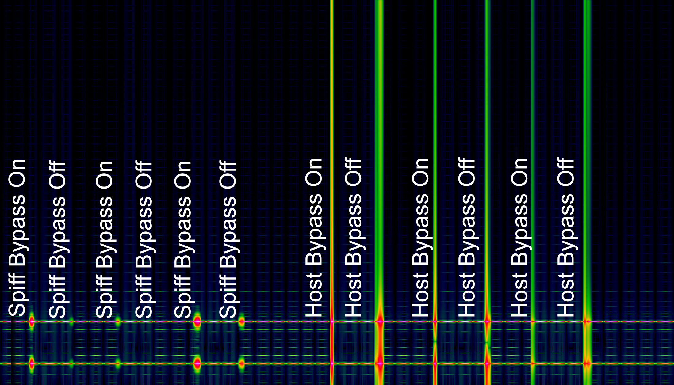
I had to be a bit more clever with this one. I setup a 1khz and 3khz sine wave that were ‘muted’ at zero crossings every n-period. This was enough to make Spiff ‘do stuff’.
I then tried with various decay settings so I could make sure Spiff was processing when I hit the bypass. From there I bypassed as normal.
The result is fantastic. It’s possible that Spiff is naturally resistant to the bypass clicks, since it is a transient (and therefore intermittent)processor. It naturally processes during sudden audio events, and bypass noise would be masked by this.
However in both testing and in listening tests it appeared that Spiff employs some sort of bypass pop protection. EXCELLENT. Great work.
Noise
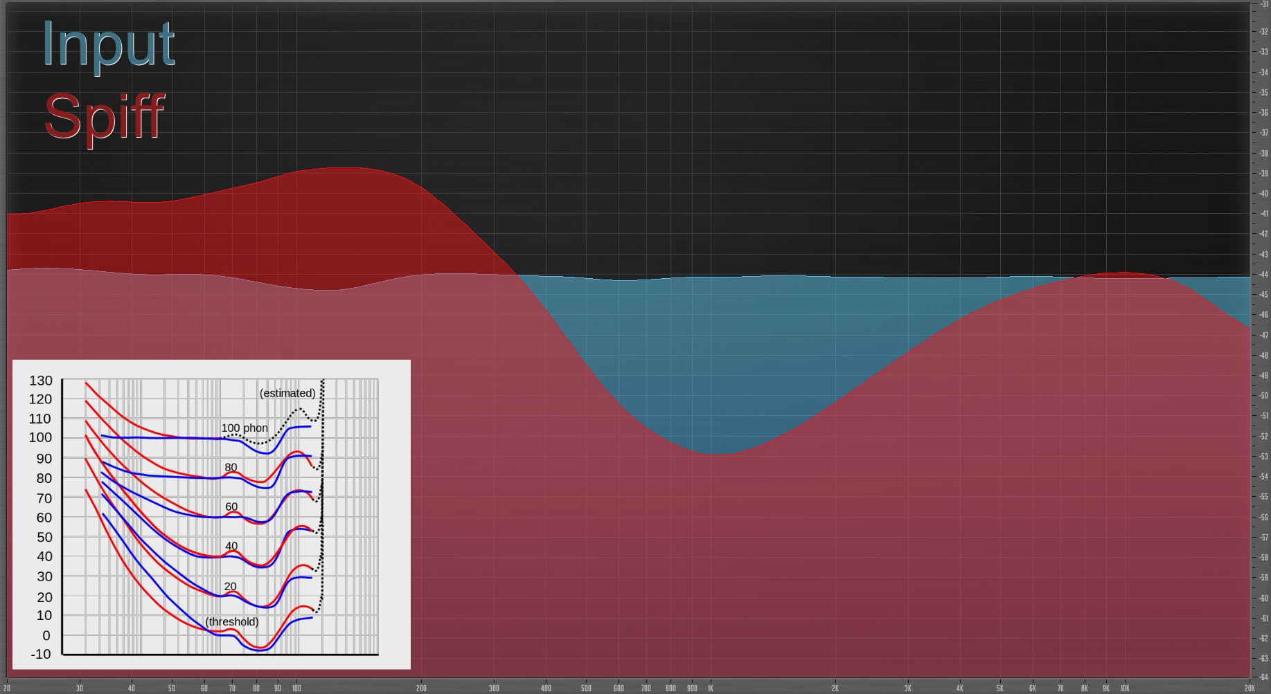
Feeding some pink noise into Spiff with depth, sensitivity and decay maxed shows something that should be familiar. (All sidechain bands were disabled)
It appears that Spiff also forms its processing to the Fletcher-Munson curve. I’ve pasted an image of this from Wikipedia into the graph above.
The depth and sensitivity knobs are similar controls, so it’s difficult to tell if one control or the other affects it more. It’s also possible that I was incorrect about Soothe’s sensitivity knob and that it’s simply ‘baked in’ to the plug-in.
So let me try something else here…
Interrupted Sweep
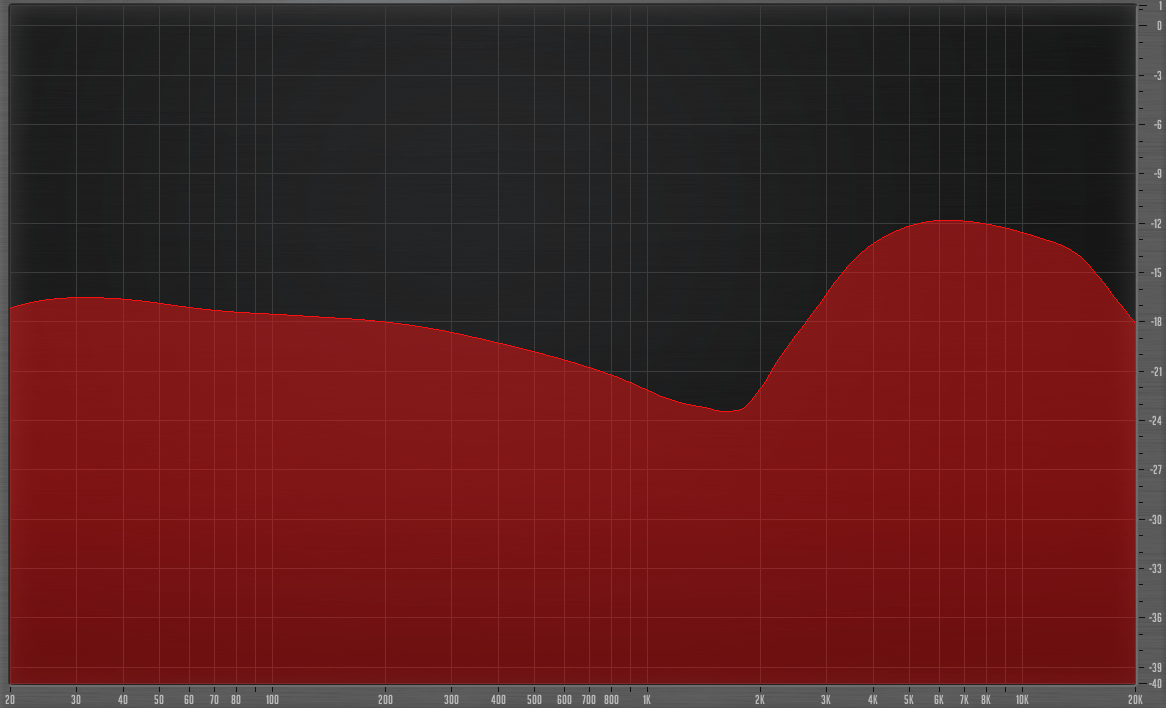
This time I setup a sine sweep that was muted 3 times a second at zero crossings (of course this doesn’t matter much since the FFT gets things wherever it wants). The sweep was 20-20,000hz at 0.1hz modulation.
This time the selectivity knob was set to 0, yet we still see the telltale curve from above. So it’s not the sensitivity, but likely part of the core filter application.
I should have done something similar with Soothe. I may have made a mistake in my analysis of Soothe in saying that the sensitivity increased the FM curve.
My apologies to Oeksound if I messed that up.
CPU
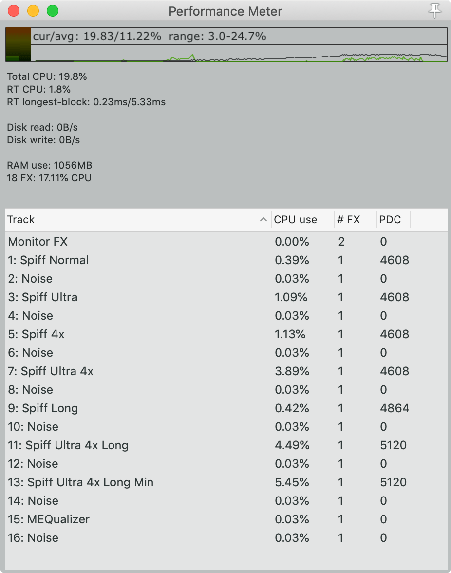
Since plain “CPU” usage numbers don’t matter, I’m showing the CPU usage relative to the freely available MEqualizer with all 6 bands active.
All processors have pink noise running into them. Spiff is setup with the default preset with sensitivity 10.
Spiff can be quite the CPU eater. With a long window, ultra resolution, 4x oversampling and minimum phase filters, Spiff can eat up nearly 182x the CPU of a simple equalizer.
Spiff, unlike Soothe, seems to benefit from these CPU eating options. There are mort certainly times where I found that ultra resolution, 4x oversampling and minimum phase filters were the optimal sound. I have a monster system and I can only run about 20 of Spiff with the settings that I can run well over 4,000 MEqualizers.
Scare-tactics aside it’s unlikely that you’ll need to ever run 20 Spiffs. Even running 2 is unlikely. If you’re finding that you have more than 2 in a project then you’re probably doing something very wrong, or some dumbass professional colleague sent you files that were not appropriate for the audio task at hand.
Real World
Peter picked five perfect blue peppers before Patrica pulled peters pants past peters feet.
So let’s get this straight. I’m not trying to show you a good mix here (cause it ain’t). I’m also purposely using some less than stellar recordings. Drums are just overheads. Bass is direct. Guitar is direct with Axiom’s auto-wah
There is no processing on these tracks. There is no level adjustment other than the comparator normalizing them -20lufs. The normalization is a bit tricky here with a transient processor. The “cut” files will sound louder than the boost files.
When listening to these you should try to hear the differences between the normal, cut and boost. I tried to go a bit beyond what I’d consider optimal so that you can easily identify what’s happening.
Conclusion
Spiffy is really spiffy. I found it potentially useful on nearly everything.
It’s more transparent than compression when trying to fix some peaky bits on musical instruments. It’s less intrusive than static EQ, or even dynamic EQs.
It works magic on singing/speech with a somewhat, uh… expressive singer. (The kind leaves globs of saliva on the mic after a performance).
I felt that Soothe was mildly situational. There are definitely people out there that may not benefit from Soothe, though it is indispensible for a number of workflows.
Spiff on the other hand, I find to be universally useful. Even with synthesized sounds, where you generally have a great deal of control over the source, I was able to use Spiff to enhance the sound in extreme ways that I could not emulate with synthesis alone.
Spiff isn’t my favorite transient processor for music. That is still Couture. A number of other ‘normal’ transient processors can be set with extreme settings and still produce useful results. Spiff becomes a bit warbly and unpleasant sounding at the extremes.
That’s a good thing though. Spiff can do things at low/moderate settings that you can’t do with any other transient processor. Spiff also excels when dealing with vocalized sounds in a way that very few things can match.
If you have a favorite transient processor then Spiff isn’t going to overlap with that much.
I’ve seen people ask if Spiff is ‘just a dynamic EQ’. It’s not. That much should be clear. Spiff doesn’t work based on thresholds. Spiff works based on energy. It’s a completely different concept from a threshold based system.
If you have a favorite dynamic EQ or compressor then Spiff isn’t going to overlap with that much.
So why wouldn’t you buy Spiff? The only reason I can think of is that you haven’t saved up enough money yet.
Support Me!
This post took 29 hours to research, photograph, write and edit. If you appreciate the information presented then please consider joining patreon or paying me for my time spent bringing you quality content!
WRITTEN IN VS Code. See this post for more information.